Recently, I’ve been interviewing for a number of roles requiring experience with low level systems programming and C/C++. During the process of preparing for these interviews, I often found it quite difficult to get the right resources and knowledge. There seems to be a lot of knowledge on the internet about how to prepare for general software engineering interviews but not a lot on how to prepare for interviews that emphasize systems programming and C/C++. Hence, I’m going to use this blog post to aggregate some of the resources I found helpful during my preparation and provide my own insight into the knowledge I believe is important.

You might now be wondering how I’m even qualified to talk about this. Well, I’ll be honest, I’m certainly no expert on these topics (yet). Heck, even the great Bjarne Stroustrup, the grandfather of the C++ programming language, said he rated himself at about seven out of ten in terms of his understanding of the language. So my goal here isn’t to make the reader an expert. Instead, I hope to help an individual with decent programming experience build a road map on how to transition into a systems programming role using C++. To that end, I believe I have enough experience over the past two years interviewing at various tech companies to confidently talk about this topic at length. Hence, I’ll be using this post to summarize my process for preparing for these roles and the tidbits of knowledge I came across during this process. Note that I’ve tailored this post to be most relevant for people aiming for roles as junior/intermediate engineers so I won’t be discussing topics such as leadership/behavioral skills and knowledge on high level design patterns. Furthermore, I also won’t be discussing the common algorithm and system design preparation that is recommended for most general software engineering interviews; I found there are plenty of guides on these topics online already. Instead, I’ll be touching on four areas that I feel are often overlooked during preparation and how I went about studying for them. These four areas are General C/C++ knowledge, multi-threading concepts, debugging skills and domain knowledge.

General C/C++ Knowledge

I know it frustrates a lot of experienced developers when both C and C++ are placed in the same category as far as skills go. This is understandable as C does not contain a lot of the abstractions with regards to memory management and OOP that is common in C++. Nevertheless, I believe that having a good foundation on both languages can be immensely helpful on the job and for tackling these interviews.

The most definitive resource for getting a solid foundation of C is The C Programming Language or simply known as K&R on account of the authors Brian Kernighan & Dennis Ritchie. Although, this book is nearly 30 years old now, C hasn’t changed all that much since it’s release so it serves an invaluable resources for the fundamentals of the language with comprehensive code samples that actually work on the first try (you think I’m kidding but this is more than I can say about a lot of modern programming books these days). I think the book is short enough such that it can easily be read cover to cover. However, where it truly shines is in the problems at the end of each chapter.

In addition to K&R, I found there are a couple other additional topics in C that require some emphasis. The first of these topics is bit manipulation. I found that oftentimes, interviewers expect candidates to know how to easily set, reset and read bits from specific registers/memory addresses along with some basic bit twiddling hacks. I suggest reviewing the following Stanford Article on some neat tricks as well as doing the top rated bit manipulation problems on a platform like Leetcode in preparation for these types of questions. Other C-based concepts I found that come up during interviews is the difference between big endian and little endian systems, the size of basic data types, representations of signed/unsigned numbers using 2’s complement and floating point representation. To better understand floating point in particular, I found that this Wikibooks article to be a good introduction to the topic along with this article, which contains a good discussion on the issues around floating point precision. In terms of data type size familiarity and endianness, I found that these topics become especially important if you are asked to code up a solution for a problem on your personal system. For example, one situation where this consideration really came to bite me was when I made the incorrect assumption that the char datatype is unsigned on all platforms during a live coding interview. Turns out, the signedness of the char datatype is actually “implementation defined” and macOS explicitly chooses to make it signed. Of course, I could have easily avoided this pitfall by simply using uint8_t from the cinttypes library but the point here is that a better understanding of the types specific to your operating system can go a long way.

Preparing for C++ interviews tends to be bit trickier than C primarily due to how expansive the language has become. I recommend two books to get a good initial foundation of the language as well as an understanding of some of the newer features added to the specification. The first is Accelerated C++: Practical Programming by Example By Andrew Koerig and Barbara E. Moo. I found that this book was an excellent introduction to iterators (chapter 5), the STL (chapters 6 & 7), template programming (chapter 8 & 9), class-based polymorphism (chapter 13) and memory management via reference counting (chapter 15). Chapter 13 is especially important as it introduces the principles behind inheritance and virtual functions, which tend to come up a lot during interviews. Similar to K&R, this book is filled with fully functional code samples and simple exercises at the end of each chapter to reinforce learning.

The second book is geared more towards understanding the new features introduced in C++11/C++14 and reads less like a tutorial and more like a reference manual. Hence, I found this book particularly dense and occasionally found myself referring to StackOverflow and various blog posts to better understand the reasoning behind some of the more sophisticated features described. Assuming that you are using this book primarily to prepare for an upcoming interview, I suggest focusing on only a select few chapters and skimming the rest. Specifically, I found that chapters 1, 2, 4 and 5 were the most useful. Chapter 1 and 2 go over the type deduction rules for C++ and discuss best practices for using the auto keyword. Chapter 4 discusses the different types of smart pointers. I suggest really understanding the internal data structures used to implement the different types of smart pointers and possibly reviewing the sample implementation from chapter 13 of Accelerated C++ for better insight. Finally, chapter 5 introduces new features around lvalues and rvalues. I found that it helpful to read this article to get the necessary background on the two value categories before jumping into this chapter.

Multithreading Concepts

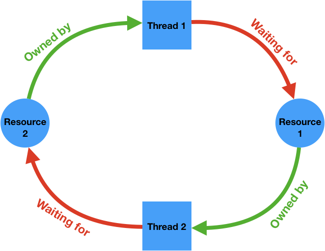
I was fortunate to have a decent background in multithreading and concurrency due to the operating systems courses I took during my undergrad. As a result, I was already quite familiar with basic synchronization primitives like semaphores and mutexes and had significant exposure to more modern mechanisms like concurrent and serial dispatch queues found in libdispatch/GCD. I also had some basic experience resolving dead locks and live locks in a production codebase, which came in particularly useful for the more theory-based problems posed during the interview process. However, I soon realized that the types of coding problems that I was assessed on tended to be more academic in nature. In order to prepare for these types of questions, I went through all the concurrency problems on Leetcode (there aren’t many) and then attempted some of the problems in the first four chapters of The Little Book of Semaphores. One basic design pattern that I found is often tested in this area is the basic producer-consumer pattern, which shows up a lot in event-driven programs (i.e. network loading).

During my practice, I’ve found that it is best to familiarize yourself with the synchronization primitives in the Standard C++ Library over other platform-specific libraries like POSIX when preparing for interviews. This is primarily because not all coding assessment platforms support POSIX so it’s best to go with the more portable library and prevent having to waste time looking up APIs during the interview. The Standard Library also has various abstractions to avoid some of the common pitfalls of multithreading programming. One example is the unique_lock, which when initialized with a mutex, automatically releases the mutex when going out of scope. Familiarizing myself with the Standard Library’s multithreading capabilities also meant that I had to become comfortable with the usage of condition variables over semaphores, which tends to be what is taught in school for thread signaling. Nevertheless, I soon discovered that both tools can be used almost interchangeably in most scenarios. A final thing to note here is that I was never asked about the more advanced synchronization features in the Standard Library such as futures, tasks or atomic objects so I don’t believe it is essential to practice using these features before an interview.

Debugging Skills

One of the most valuable skills I learned in my first job is how to debug issues in a large codebase effectively. The importance of this skill generally isn’t stressed enough in school but I suppose that is understandable as students aren’t expected to maintain a large codebase year round. Nevertheless, I found that my knowledge of this topic was evaluated in some unexpected ways during the interview process often in the form of hypothetical scenarios or in the behavioral interview. Hence, I found it useful to establish a general high-level framework for debugging some of the issues that may pop up when working on a large codebase. The two areas I have the most experience debugging is general programming errors and memory-related issues so I’ll try to outline the general systematic approach I’ve devised to tackle each of them.

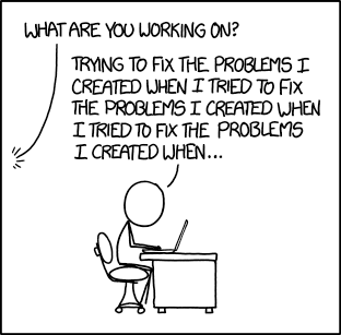
I often refer to general programming errors as situations where the program behaves contrary to expectation due to a logical oversight during design or implementation. The first step when debugging these types of issues is understanding the correct behaviour and the current unexpected behaviour. Often this step requires carefully reading through the originator’s bug report and analyzing any provided logs. The log analysis often involves tracking object lifecycles to determine the state of the system during the point of failure. Occasionally, a bug can be fully diagnosed and fixed at this stage itself if one has sufficient familiarity with the problem area. However, in most cases, if this truly is a result of a programming oversight, there probably isn’t enough logging to root cause the issue at this stage. At this point, the next step is to try and reproduce the problem locally with some extra logging or with a debugger using hints from the log/bug report. If this issue is suspected to be a regression in behaviour, it is often helpful to attempt to reproduce the bug with different versions of the software and look for differences in logging to diagnose any unexpected state changes in the system. This step is often times the most laborious part of the entire process especially if the bug is a concurrency or network-related issue with a low rate of reproducibility. Once the problem is sufficiently understood and can be manually reproduced with relative ease, the next step would be to write a unit test to consistently reproduce the issue. This step can be tempting to skip but is invaluable for verifying that any code changes that you devised or was suggested during the code review actually fixes the issue at hand. The unit test also serves as a safety net to prevent future regressions and is an excellent source of documentation if at any point you have to revisit the issue at a later date. When developing the actual fix for the issue, it is important to assess the code change for risk of causing any new regressions in behaviour, which is where automated testing comes into play. However, if the fix requires altering an integral low level system component, it may still be a good idea to tailor the fix to be as minimally intrusive as possible with extra logging just in case. It may also be useful to try to relate the bug to other similar issues encountered and propose a more large scale system refactor to prevent such errors from occurring in the future.

Your effectiveness when it comes to debugging memory-related issues is dependent primarily on your mastery of the associated tooling. Using a tool such as Valgrind on Linux or Instruments and memgraphs on Apple platforms while reproducing a memory issue can be very helpful in identifying objects of interest for further investigation. One such practice I’ve engaged in quite often is logging memory addresses for objects of interest and cross correlating these addresses with a leaks or allocations trace from Instruments. This is an effective way to obtain a full retain/release history of specific segments of memory and is much easier than manually adding instrumentation to track object ownership lifecycles in a reference-counted environment. I’ve also found that being able to carefully read thread stack traces in crash and Jetsam reports to be pretty useful in quickly diagnosing some obvious memory issues (i.e. processes spawning too many blocked threads). Generally speaking, I’ve tried to employ the same procedure I use for general programming errors for memory-related issues as well with the addition of tooling.

Domain Knowledge

Domain knowledge tends to be emphasized more during the system design interview for specialist SWE roles. I found the best way to prepare for these interviews is to review any design documents or tech talks available to you to get an idea of some common design considerations behind systems of interest. For example, when interviewing for a position on a video/multimedia-related team, it maybe useful to have a high level understanding of the data flow for audio/video playback from the hardware abstraction layer to the client application on an established platform such as Android. A good operating systems background can help in understanding some of the design trade offs for these systems but areas of emphasis are usually based on your experience or the requirements for the role. For example, some concepts that came up during my interviews were different types of memory allocation algorithms, types of common hashing functions, methods for interprocess communication, network socket programming, interrupt service routines and system daemon design. I haven’t found a definitive book to prepare for all of these topics due to their somewhat disparate nature but will be sure to update this section once I come across some study resources that maybe helpful here.

Congrats on making it past the previous post. That last post was pretty theory heavy and covered a lot of ground on Monte Carlo Methods. For this blog post, I’m going to pick up the pace a little bit and cover some more fundamental RL algorithms. In fact, by the end of this post, you should have a decent theoretical and practical understanding of the Dueling DDQN algorithm.  Again, I’ve gathered most of this information from reading research papers on DQN, watching David Silver’s RL course and reading Sutton and Barto.

Throughout this post, I’ll be building upon an implementation of this algorithm in python to give you more insight into the finer details. After every code snippet, I’ll try to explain some of the lines that may be difficult to understand or are key to the underlying algorithm. During these sections, I find it most helpful to open up this blog post in another tab and go through the code line by line with my explanations. I’ve adopted this methodology from Trask’s blog post on implementing neural networks with numpy (which by the way, I highly recommend going through if you’re serious about this stuff). Aside from that, you can be sure to find full implementations of any of the algorithms I discuss in this post and in my previous posts on my GitHub.

Q-Learning

So let’s begin with the vanilla Q-learning algorithm using simple table look up methods. How does this algorithm work? Well, Q-learning is a simple off-policy learning method based off of the idea of bootstrapping. Bootstrapping is the idea that new estimates can be made from previous estimates. This idea is different from Monte Carlo Methods (MCM), which were discussed in detail in the previous post. In MCM, the agent bases its policy updates on only the returns obtained from the most recent episode. However, in this case, the Q-learning algorithm performs policy updates after every step taken in the environment rather than all at once at the end of an episode. This means the algorithm is more adaptive to changes in the environment and less susceptible to the high variance involved with updating the policy on only a single experience trajectory. Q-learning along with all algorithms that use bootstrapping to perform the generalized policy iteration (GPI) technique  are identified as temporal difference methods.

Mathematically, in Q-learning the updates to the Q-values are performed using Equation 1 while in MCM, the update operation looks more like equation 2.  The key difference here is that with Q-learning, the update operation is applied online, when the entire discounted return from a specific time step () is not yet available to the agent. Instead, the agent approximates this value by using the current reward, along with the discounted maximum Q-value available in the next state, . Remember that the Q-value represents an estimate of the total expected reward that the agent can get if a specific action is taken in a particular state. Hence, the max over the Q values represents optimal behavior from that point onwards. The sum of  current reward and discounted maximum Q-value in the next state corresponds to the Temporal Difference (TD) target or the value that you want the current Q value to move towards.  This TD target represents the value of taking an action, and acting optimally in regard to the current policy until the end of the episode. Similarly, the TD error represents the difference between the TD target and the current Q-value (). Equations 1 and 2 contrast the update rules used for Q-learning and MCM.

Equation 1: Q-Learning Update

or equivalently,

Equation 2: Off-policy MCM Update

Another thing to notice here is that I don’t have to worry about importance sampling ratios () for Q-learning as I’m not using the entire experience trajectory for the policy evaluation step. Instead, the agent is performing Q-value updates online with just one extra step of information. This is why you will not see the importance sampling ratio,  show up in the Q-learning update. To illustrate this point pictorially, have a look at Figure 1.

Figure 1: Comparing MCM Updates (left) with TD updates (right) for decision-making. Taken from Lecture 4 of David Silver’s excellent introductory RL course.

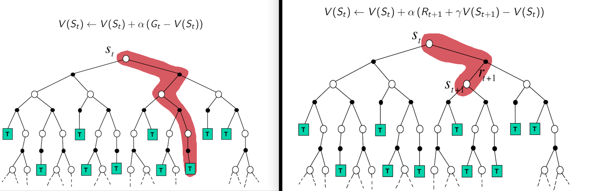
Note: The above images uses or state-values rather than the or state-action values used in Q-learning. Nevertheless, the update rules for state values and state-action values are still more or less the same.

Let’s see how this looks like in code.

def q_learning(env, num_episodes, discount_factor=1.0, alpha=0.5, epsilon=0.1):
    """
    Vanilla Q-Learning algorithm: Off-policy TD control. Finds the optimal greedy policy
    while following an epsilon-greedy policy

    Args:
        env: OpenAI environment.
        num_episodes: Number of episodes to run for.
        discount_factor: Gamma discount factor.
        alpha: TD learning rate.
        epsilon: probability of sampling a random action, a float value betwen 0 and 1.

    Returns:
        A tuple (Q, episode_lengths).
        Q is the optimal action-value function, a dictionary mapping state -> action values.
        stats is an EpisodeStats object with two numpy arrays for episode_lengths and episode_rewards.
    """

    # A nested dictionary that maps state -> (action -> action-value)
    Q = defaultdict(lambda: np.zeros(env.action_space.n))

    # The policy we're following
    policy = make_epsilon_greedy_policy(Q, epsilon, env.action_space.n)

    for i_episode in range(num_episodes):
        done = False
        s = env.reset()

        while not done:
            action = np.random.choice(np.arange(env.action_space.n), p=policy(s))
            new_s, r, done, _ = env.step(action)
            Q[s][action] += alpha * (r + discount_factor * np.max(Q[new_s]) - Q[s][action])
            s = new_s

    return Q

Some things to note here:

Line 23: the make_epsilon_greedy_policy function holds a reference to the Q table/function and returns a function (policy). This returned function when invoked,  returns a probability distribution over possible actions in each state (-greedy policy).

Line 33: Most of the magic for this algorithm happens in this line. If you carefully examine it, you’ll notice it’s exactly the same as Equation 1 from before.

Deep Q-Learning (DQN)

This all seems pretty reasonable right? But by now I bet you’re wondering where the deep in deep reinforcement learning come in. Before I get to that let’s go back to the previous algorithm for a bit and examine one its biggest flaws. What’s this flaw you ask? Well, imagine a problem with a million discrete states or a continuous state space. Now imagine training this algorithm in this environment and storing each of the state-action values. It doesn’t take a genius to realize that you’re quickly going to run out of memory without getting very far in the training process. So how do we make this algorithm more scalable? Well let’s add our favorite buzzword and mathematical blackbox, the neural network, into the mix. Brace yourself as we’re now entering deep RL territory.

The major difference here is that instead of querying a table to obtain the Q-value associated with each state-action pair, we’re going to be using a neural network to approximate it. This neural network will take the current state and output a set of Q values associated with each action that the agent can take in the current state.

However, there are still a couple of small changes we have to make to incorporate the neural network into the Q-learning algorithm. Specifically, we need to introduce the concept of a target network and experience replay to stabilize the training process. One of the major differences in the use of neural networks in reinforcement learning as opposed to supervised learning, is that the target output isn’t stationary. This is because as the agent explores the environment, it iterates on its policy and changes it’s Q-values accordingly. Moreover, training a neural network on such a highly non-stationary target would quickly lead to instability (imagine chasing a moving bus as opposed to a stationary one). To address this issue, many implementations of the Deep Q-learning (DQN) algorithm use two Q-networks. The first network is updated after every time step using back propagation as usual (the working network) and the other network is used exclusively to predict the TD target (the target network). In this case, the target network serves as a semi-stationary target as it is updated less frequently than the working network. Moreover, whenever the target network is updated, the update process simply involves copying the weights from the working network.

The other technique that’s used to aid in stability is experience replay. Experience replay is a technique where the agent explores the environment while maintaining a buffer of state transitions. This buffer of experience is then randomly sampled and the resulting samples are used to perform the generalized policy iteration. But why would anyone opt to do this instead of just using the most recent transitions? Well, that idea may work for tabular Q-learning, but it’ll likely lead to stability issues when non-linear function approximators like neural nets are used to learn the Q-function. These stability issues arise from multiple convergence proofs that require neural networks be trained on independently and identically distributed data (i.i.d. data). By training a model on continuous transitions, there exists strong correlations between samples, which clearly violates the i.i.d. requirement. This issue can be remedied by using experience replay and randomly selecting a batch of previous state transitions for training. Furthermore, this technique also enables the network to train on the same state transition multiple times, which aids in generalization.

So how does this all look like in practice? Let’s go through an implementation.

def deep_q_learning(sess,
                    env,
                    q_estimator,
                    target_estimator,
                    n_steps,
                    replay_memory_init_size=64,
                    epsilon_decay_size=1000,
                    replay_memory_size=10000,
                    update_target_estimator_every=100,
                    discount_factor=0.99,
                    batch_size=32):
    """
    Q-Learning algorithm for off-policy TD control using Function Approximation.
    Finds the optimal greedy policy while following an epsilon-greedy policy.

    Args:
        sess: Tensorflow Session object
        env: OpenAI environment
        q_estimator: Estimator object used for the q values
        target_estimator: Estimator object used for the targets
        n_step: Number of steps to run for
        replay_memory_size: Size of the replay memory
        replay_memory_init_size: Number of random experiences to sample when initializing the reply memory.
        update_target_estimator_every: Copy parameters from the Q estimator to the target estimator every N steps
        discount_factor: Gamma discount factor<span id="mce_SELREST_start" style="overflow:hidden;line-height:0;"></span>
    """
    # The replay memory
    replay_memory = []

    epsilon_start = 1.0
    epsilon_final = 0.01
    epsilon_decay = 1000

    epsilon_by_frame = lambda frame_idx: epsilon_final + (epsilon_start - epsilon_final) * math.exp(-1. * frame_idx / epsilon_decay)

    epsilons = [epsilon_by_frame(i) for i in range(10000)]

    policy = make_epsilon_greedy_policy(q_estimator, env.action_space.n)

    done = True
    total_t = sess.run(tf.contrib.framework.get_global_step())

    losses = []
    for i in range(replay_memory_init_size):
        epsilon = epsilons[min(total_t, len(epsilons)-1)]
        if done:
            state = env.reset()
            action = np.random.choice(range(env.action_space.n), p=policy(sess, state, epsilon))
        else:
            action = np.random.choice(range(env.action_space.n), p=policy(sess, state, epsilon))
            state = next_state
        next_state, reward, done, _ = env.step(action)
        replay_memory.append((state, action, reward, next_state, done))
        total_t += 1

    loss = None

    for step in range(n_steps):

        if done:
            state = env.reset()

        epsilon = epsilons[min(total_t, len(epsilons)-1)]

        if total_t % update_target_estimator_every == 0:
            copy_model_parameters (sess ,q_estimator ,target_estimator)

        action = np.random.choice(range(env.action_space.n), p=policy(sess, state, epsilon))
        next_state, reward, done, _ = env.step(action)

        if len(replay_memory) == replay_memory_size:
            replay_memory.pop(0)

        replay_memory.append((state, action, reward, next_state, done))

        minibatch = random.sample(replay_memory, batch_size)

        minibatch_states, minibatch_actions, minibatch_rewards, minibatch_next_states, minibatch_dones = map(np.array, zip(*minibatch))

        max_Qs = np.max(target_estimator.predict(sess, minibatch_next_states), axis=1)
        targets = minibatch_rewards + (1 - minibatch_dones) * discount_factor * max_Qs

        # use loss and do backprop update on neural network estimator
        loss = q_estimator.update(sess, minibatch_states, minibatch_actions, targets)

        state = next_state
        total_t += 1

At first glance, it looks a lot more complicated than the tabular Q-learning algorithm but honestly, it isn’t all that different. The main difference is I’m now using a machine learning library (TensorFlow) to iterate on my Q-networks (q_estimator and target_estimator) rather than just directly changing values in a Q-value store. The q_estimator and target_estimator objects are just instances of a custom Estimator class. This estimator class pretty much encapsulated a TensorFlow model used for training.

lines 30-37: these lines just declare a list of epsilon values and aren’t really specific to the algorithm. I just found that decaying epsilon by worked pretty well in practice.

lines 38: defining my epsilon greedy policy. This function stores a reference to the q_estimator, which is the working Q-network.

lines 44-54: I’m just initializing the replay buffer with some state transitions from the default policy before I start the actual training. Nothing too special here either.

lines 65-66: Now we’re getting into the meat of the algorithm. As I mentioned before, for this implementation, I have two networks (working and target). After update_target_estimator_every number of steps, I copy over the weights from my working network into the target network. This way the target network remains somewhat stationary during the training process and is updated only occasionally.

lines 68-69: Nothing too complicated here, I’m just sampling my -greedy policy and taking the appropriate action in the environment.

lines 71-74: After every state transition, I’m sure to add it to the replay memory. It’s important to recognize that I am treating the replay memory list like a circular buffer. So once it’s full I remove the oldest element and only keep the most recent state transitions.

lines 76-78: I now randomly sample batch_size state transitions from my replay memory to adhere to the i.i.d. data requirement that I mentioned before.

lines 80-81: Here I’m evaluating the TD target using the target network

line 84: So this function does quite a bit. Firstly, it calculates the mean square error (loss) between the TD target and the current Q-value predicted by the working network (q_estimator). Then it performs back-propagation using the AdamOptimizer to update all the weights of the working network. The details of back propagation operation are abstracted away due to Tensorflow.

…and that’s it. With this algorithm you should be able to train an agent to play several popular Atari games. But there are still some more improvements that we can make to this algorithm, which I’ll go over next.

Double Deep Q-learning (DDQN)

One of the problems with DQN is that it is prone to overestimation due to the use of the max operator in the Q-learning update (check back on Equation 1). This is a real problem especially early in the training process when all action-value estimates contain some amount of random noise. These overestimations can result in noisy actions being selected more often than the true optimal action in any given state, which in term leads to suboptimal policies. How do can we combat this issue? One idea, is to decouple the optimal action selection and the maximum Q-value selection by using two separate networks for the TD target. In other words, the agent uses one network to select the optimal action in the next state and then uses that selected action to get the maximum Q-value from another network for the TD target.

Equation 3 shows the new update rule. Notice that I’ve introduced some new notation, specifically the and symbols. These symbols are used to indicate that these Q-values are no longer just entries in a table but are rather generated from a function approximator with weights. In this case, and represent two different function approximators with their own set of weights, which are used to generate the Q-values. This new update rule effectively decouples optimal action selection from Q-value evaluation to form an unbiased estimate.

Equation 3: Unbaised Double Q-Learning Update

Let’s jump to the implementation.

def deep_q_learning(sess,
                    env,
                    q_estimator,
                    target_estimator,
                    n_steps,
                    replay_memory_init_size=64,
                    epsilon_decay_size=1000,
                    replay_memory_size=10000,
                    update_target_estimator_every=100,
                    discount_factor=0.99,
                    batch_size=32):
    """
    Q-Learning algorithm for off-policy TD control using Function Approximation.
    Finds the optimal policy while following an epsilon-greedy policy and avoiding the maximization bias by using Double Q-Learning.

    Args:
        sess: Tensorflow Session object
        env: OpenAI environment
        q_estimator: Estimator object used for the q values
        target_estimator: Estimator object used for the targets
        n_step: Number of steps to run for
        replay_memory_size: Size of the replay memory
        replay_memory_init_size: Number of random experiences to sample when initializing the reply memory.
        update_target_estimator_every: Copy parameters from the Q estimator to the target estimator every N steps
        discount_factor: Gamma discount factor<span id="mce_SELREST_start" style="overflow:hidden;line-height:0;"></span>
    """
    # The replay memory
    replay_memory = []

    epsilon_start = 1.0
    epsilon_final = 0.01
    epsilon_decay = 1000

    epsilon_by_frame = lambda frame_idx: epsilon_final + (epsilon_start - epsilon_final) * math.exp(-1. * frame_idx / epsilon_decay)

    epsilons = [epsilon_by_frame(i) for i in range(10000)]

    policy = make_epsilon_greedy_policy(q_estimator, env.action_space.n)

    done = True
    total_t = sess.run(tf.contrib.framework.get_global_step())

    losses = []
    for i in range(replay_memory_init_size):
        epsilon = epsilons[min(total_t, len(epsilons)-1)]
        if done:
            state = env.reset()
            action = np.random.choice(range(env.action_space.n), p=policy(sess, state, epsilon))
        else:
            action = np.random.choice(range(env.action_space.n), p=policy(sess, state, epsilon))
            state = next_state
        next_state, reward, done, _ = env.step(action)
        replay_memory.append((state, action, reward, next_state, done))
        total_t += 1

    loss = None

    for step in range(n_steps):

        if done:
            state = env.reset()

        epsilon = epsilons[min(total_t, len(epsilons)-1)]

        if total_t % update_target_estimator_every == 0:
            copy_model_parameters (sess ,q_estimator ,target_estimator)

        action = np.random.choice(range(env.action_space.n), p=policy(sess, state, epsilon))
        next_state, reward, done, _ = env.step(action)

        if len(replay_memory) == replay_memory_size:
            replay_memory.pop(0)

        replay_memory.append((state, action, reward, next_state, done))

        minibatch = random.sample(replay_memory, batch_size)

        minibatch_states, minibatch_actions, minibatch_rewards, minibatch_next_states, minibatch_dones = map(np.array, zip(*minibatch))

        max_actions = np.argmax(q_estimator.predict(sess, minibatch_next_states), axis=1)
        targets = minibatch_rewards + (1 - minibatch_dones) * discount_factor * target_estimator.predict(sess, minibatch_next_states)[np.arange(len(minibatch_actions)), max_actions]

        # use loss and do backprop update on neural network estimator
        loss = q_estimator.update(sess, minibatch_states, minibatch_actions, targets)

        state = next_state
        total_t += 1

If you look carefully, not much changed aside from two lines for code.

Lines 80-81: Here I’m explicitly determining the best action using q_estimator or the working network and using this selected action to evaluate the associated Q-value using the target network. Finally, this Q-value is used in the TD target calculation.

Dueling Double Deep Q-Learning (DDDQN)

I know what you’re thinking, that’s a lot of D’s but I promise this is the last one. So where does the last D come from? Well, the problem that DDDQN tries to tackle is that of generalizability. One insight that a recent research paper made is that for many reinforcement learning tasks, there exists many states where the action taken does not not impact the next state all that much (i.e. switching to the left of right lane when the road ahead is clear). Nevertheless, the network still has to learn to differentiate between these two Q-values. To give the network an easier time in identifying such situations, it was proposed to have the network output two values rather than just one.  These two separate values would be a state-value, representing the value of being in a particular state and an advantage value, which would represent the added value of taking a particular action in that state. How does this address the issue of generalizability? Well, by decomposing the  Q-value into state and advantage, more of the network is regularly updated through the value stream as updates can be performed after every state visitation. Ultimately,  combining state and advantage approximations leads to a better estimations of the Q-value.

However, implementation-wise this may seem odd. How does one get a neural network to output two separate but related values? The idea is to have one common layer for the input and two branching sets of neural network layers to estimate the state-value and advantage separately. Then simply sum these two values to end up with the more familiar Q-value estimate. Equation 4 demonstrates this relationship.

Equation 4:  Q-value Decomposed into State-value and Advantage

# Placeholders for our input
self.X_pl = tf.placeholder(shape=(None, state_dim), dtype=tf.float32, name="X")
# The TD target value
self.y_pl = tf.placeholder(shape=(None,), dtype=tf.float32, name="y")

self.weights = tf.placeholder(shape=(None,), dtype=tf.float32, name="weights")

self.actions_pl = tf.placeholder(shape=(None,), dtype=tf.int32, name="act")

batch_size = tf.shape(self.X_pl)[0]

self.fcl1 = tf.layers.dense( self.X_pl, 128, activation=tf.nn.relu, name='fcl1')

if deulling is True:
    # value prediction layers
    self.fcl2_value = tf.layers.dense( self.fcl1, 128, activation=tf.nn.relu, name='fcl2_value' )
    self.value_prediction = tf.layers.dense( self.fcl2_value, 1, name='fcl3_value')

    # advantage prediction layers
    self.fcl2_advantage = tf.layers.dense( self.fcl1, 128, activation=tf.nn.relu, name='fcl2_advantage')
    self.advantage_prediction = tf.layers.dense( self.fcl2_advantage, action_space, name='fcl3_advantage')

    self.mean_advantage = tf.reduce_mean(tf.reduce_mean(self.advantage_prediction))
    self.predictions = self.value_prediction + (self.advantage_prediction - self.mean_advantage)
else:
    self.fcl2 = tf.layers.dense( self.fcl1, 128, activation=tf.nn.relu )
    self.predictions = tf.layers.dense( self.fcl2, action_space )

Conclusion

Due to overwhelming demand, I figured I should make more of an introductory post about some of the motivations for reinforcement learning and introduce some basic terminology, which I will be using throughout the rest of this blog series. I’ll try to keep this post  relatively accessible but I do assume at least a basic understanding of machine learning and statistics. Alright then, without further ado, let’s get started!

Inspirations

Reinforcement learning is an approach to machine learning, which is concerned with goal-directed behavior. The types of problems that reinforcement learning tackles are very different from the other two more common paradigms of machine learning, which are supervised and unsupervised learning. Specifically, the goal of reinforcement learning is to derive the optimal policy or pattern of behavior for a control problem.

This paradigm is heavily modeled after biological systems and reward-based learning found in psychology. In fact, the pioneer of reinforcement learning, Richard S. Sutton, did his undergraduate degree in psychology and not computer science (although I don’t really recommend this if you want to purse a job outside academia). In fact, many of his high-level ideas can be traced back to operant conditioning, which is an idea that behavior can be influenced with rewards and punishments.

Multi-armed bandits

To concretely illustrate the type of problem that reinforcement learning attempts to solve, let’s go through a popular example and gradually build upon it. Imagine that there are slot machines at a casino. Each of these slot machines gives varying amounts of reward corresponding to a specific probability distribution. How can one get the most money back by gaming this system? Well, the best way is to simply try each of the slot machines () times and use the obtained reward at each time step, to generate an expected reward estimate for each machine, . In other words, you would continuously improve upon your reward estimates with your incremental update rule looking something like the following:  .  After a sufficient number of tries, you should be pretty confident on which machine gives the most reward. At this point, you can stop exploring and just continue to pick the slot machine that gives the most expected reward (disclaimer: don’t try this at an actual casino). In other words, you are now acting greedily with respect to the information that you know by just picking the best option every time. This problem, as it currently stands, is known as the traditional multi-armed bandit problem.

Now, what if those same reward probabilities are gradually changing with time (i.e. non-stationary). Well in this case, it would be wise to introduce the idea of discounting with a new parameter,  also known as the discount rate. This idea puts more emphasis on newer rewards to account for the inherent non-stationary nature of the environment. The incremental reward update for each slot machine now looks more like the following:  . The experienced observer will notice that this update rule forms the basis of all further reinforcement learning algorithms. However, we still haven’t even introduced all of the complications of the generic RL problem.

So let’s continue by adding another wretch in the the traditional multi-armed bandit problem. Now imagine that the probability of getting a reward from each slot machine is changing dynamically after each play. In fact its changing so much that simply discounting the reward signal isn’t enough to come up with the best strategy. This means that every time you pick a slot machine, it’s like all of the previous machines are replaced with new ones; you’ve essentially arrived at a new state. The assumption now is that any immediate action taken impacts both the immediate reward along with the next state. In this case, the goal is to learn a policy, of picking slot machines rather than just determining the optimal machine to pick every time. We’ve now reached the full reinforcement learning problem.

The RL Problem

Now that you have a rough idea of how this all works, let’s try to generalize these ideas a bit more. All reinforcement learning problems can be broken up into a series of states, where an agent can perform a single action, from a set actions and receive a single scalar reward,  before transitioning into another state,  . The probability of transitioning into any given state and obtaining a reward is conditioned ( ) only on the previous state and action, . In other words, the information found in any state is sufficient for making a prediction about the next state. This requirement is known as the Markov property.  This stochastic process defined by states, actions and rewards is known as a Markov Decision Process (MDP). Hence, the ultimate goal of a RL algorithm is to come up with a method for picking actions at each state or a policy, such that the cumulative reward is maximized.

This all seems simple enough until you take into account the credit assignment problem. That is, how does one properly  assign credit to each action that one takes within an MDP? This is a difficult question to answer as many seemingly suboptimal actions taken at the current time step can have significant pay off later on. Many reinforcement learning algorithms attempt to back-up some of these reward signals and gradually learn  more about the underlying dynamics of an environment through direct interactions with it. This is done by either incrementally iterating upon the value of a state following a certain policy, or the value of being in state and taking a particular action, .

Another difficulty in reinforcement learning comes from addressing the exploration-exploitation problem. This problem deals with balancing the requirements of picking the best action with respect to the current knowledge of the environment or continuing to explore the state-space to come up with better actions in the future. This issue is especially tricky if the state space is very large or continuous. Many algorithms address this issue by introducing some stochasticity into the decision-making process or by using function approximators (i.e. neural networks).

By now you’re probably wondering, how do we solve these problems and where do they actually show up in the real world? Well, I’ll probably need a couple more blog posts to answer the first question but I’ll try to answer the second one in the next section.

Applications

The power of RL versus more classical methods for control comes from its generalizability and scalability when combined with neural networks. David Silver first proved this point by showing a deep RL agent perform above  human capabilities on a number of classic Atari games (you can read more about it here). His research proved that reinforcement learning can be applied to many simple games to learn optimal behavior. However, the applications don’t end there. In fact, reinforcement learning can be applied to any decision-making process where the environment can be at least partially represented as an MDP.

Here are some more examples:

• A stock-trading agent that will improve its strategy for trading  through experience alone (paper) or alternatively an agent that learns to trade specifically in cryptocurrencies (I can hear all the SV VCs fawning already)
• A RL agent that learns to adapt to difficult network conditions to deliver the best quality of experience for a user watching streamed video content (paper)
• A RL agent that acts as the flight controller for an autonomous helicopter (paper)
• A RL agents used to control a manufacturing robot that performs generalized automation tasks (paper)

I could go on but suffice to say, the applications of reinforcement learning are diverse and varied.

Conclusion

I hope this post has given you a gentle introduction to reinforcement learning. In the next couple of posts, I’ll be covering some foundational knowledge on RL along with some popular algorithms applied to some interesting problems. If there are any inaccuracies in this post or if you have general feedback for me, feel free to shoot me an email or leave a comment below 🙂

This will be the first post in a series of blog posts where I’ll try to cover some of the fundamental ideas behind some basic reinforcement learning algorithms. Throughout this series, I will refer to some of the intuition behind certain key elements incorporated into these algorithms and provide some simple python implementations tested on OpenAI’s gym package. I will start by covering tabular methods for RL and in later posts move onto algorithms that use neural networks for function approximation. Most of the information found in this series can be obtained by reading Andrew Barto and Richard S. Sutton’s excellent Introduction to Reinforcement Learning textbook, which is freely available to all. Personally, I’ve watched most of  the lectures from David Silver’s RL UCL course and worked a couple exercises found in the Pratical_RL GitHub course and Denny Britz’s RL repository. Occasionally, I may refer to other resources, which I will be sure to note down when necessary. All the code used in this blog plot post is freely available on my Github.

I assume that readers of this blog have taken a basic statistics course and have a high-level understanding of reinforcement learning (i.e. know the definitions of a reward, normal distribution, Markov Decision Process, etc). If not, I may go over some of these topics in another blog post. However, I imagine the ideal reader for this blog series is somewhat like me when I first encountered reinforcement learning. That is, a wide-eyed undergraduate student with a basic understanding of formal mathematics/statistics, some decent software engineering experience and a lot of extra time on their hands.

So on to the topic at hand, Monte Carlo learning is one of the fundamental ideas behind reinforcement learning. This method depends on sampling states, actions and rewards from a given environment. This means that one does not need to know the entire probability distribution associated with each state transition or have a complete model of the environment. Instead, as long as there exists a method to sample from the enviroment, one can use any captured experience data to learn an optimal policy over a large number of episodes. Furthermore, a policy, in the RL sense, is a way of picking actions at every state ( ).  This policy function is iterated upon after the end of every episode of experience with the ultimate goal of reaching a policy that gives the most reward on average. Note that the policy function can be either deterministic or stochastic in the way that it picks actions. However, for Monte Carlo Methods, we will assume that the policy is deterministic.

Generalized Policy Iteration

So how does this all work? Well, like more traditional dynamic programming methods for control, Monte Carlo algorithms follow the Generalized Policy Iteration (GPI) framework. This framework can be broken down into two steps; policy evaluation and policy improvement. The policy evaluation step involves iterating on Q-value estimates or state-action values based on new data obtained from completing an episode. These Q-values give a numerical value for being in a given state and taking a particular action, . Mathematically, they correspond to the expected return or expected discounted reward from taking a particular action, in state, . The return in this case is defined as where is the reward obtained immediately after state, . The purpose of discounting the reward signal with parameter is to quantify the present value of future rewards (think present value of money with inflation).

Once policy evaluation is complete the second step of GPI is the policy improvement step. This step involves improving upon the current policy () by greedily choosing the actions with the largest Q-value for each state. GPI works by continuously alternating between policy evaluation and improvement until convergence upon the optimal values and the optimal policy, .

On-policy, -greedy, First-visit Monte Carlo

The first actual example of a Monte Carlo algorithm that we’ll look at is the on-policy, -greedy, first-visit Monte Carlo control algorithm. Lets start off by understanding the reasoning behind its naming scheme. The reason why this algorithm is known as an -greedy algorithm is due to its approach in tackling the classic exploration-exploitation trade-off. This problem arises from the conflicting goals of RL, which are to both sufficiently explore the state space and behave optimally in all states. -greedy Monte Carlo algorithms approach this issue by employing a adjustable parameter, to balance these two requirements. This results in this algorithm picking a specific non-greedy action, with a probability of and the greedy action according to the current policy with a probability of . In practice, is also usually decayed over time towards a fully greedy policy. Using this method, with a sufficient number of iterations, each state-action pair in the environment is guaranteed to be explored. At the same time, the greedy action is also occasionally taken to evaluate the current policy.

The on-policy part of this algorithm addresses how this algorithm uses the same policy for state-space exploration and policy improvement. This means that the generated Q-values would only ever correspond to a near-optimal policy with some exploration. The alternative approach would be to use two policies where one would be used for exploration and the other for policy improvement. This type of algorithm is known as an off-policy method and will be described in the next section.

Finally, the first-visit aspect of this algorithm refers to how this algorithm only looks at the first time any given state, is encountered in an episode for the policy evaluation phase. This means that if the same state is visited multiple times in an episode, only the reward associated with the first visit is used to update the Q-values. The alternative approach would be an every-visit method. This approach involves updating the associated Q-values for every visit in an episode. Both these approaches have very similar theoretical convergence properties but perform differently in practice.

An implementation of the discussed algorithm in python is provided below with a line-by-line explanation following:

def mc_control_epsilon_greedy(env, num_episodes, discount_factor=1.0, epsilon=0.1):
    """
    Monte Carlo Control using Epsilon-Greedy policies.
    Finds an optimal epsilon-greedy policy.

    Args:
        env: OpenAI gym environment.
        num_episodes: Number of episodes to sample.
        discount_factor: Gamma discount factor.
        epsilon: Chance the sample a random action. Float betwen 0 and 1.

    Returns:
        A tuple (Q, policy).
        Q is a dictionary mapping state to action values.
        policy is a function that takes an observation as an argument and returns
        action probabilities
    """

    # Keeps track of sum and count of returns for each state
    # to calculate an average. We could use an array to save all
    # returns (like in the book) but that's memory inefficient.
    returns_sum = defaultdict(float)
    returns_count = defaultdict(float)

    # The final action-value function.
    # A nested dictionary that maps state to (action to action-value).
    Q = defaultdict(lambda: np.zeros(env.action_space.n))
    # A nested dictionary that maps state to (action to number of times state-action pair was encountered).
    N = defaultdict(lambda: np.zeros(env.action_space.n))
    iterations = 0
    # policy improvement: this function holds a reference to the Q_values
    policy = make_epsilon_greedy_policy(Q, epsilon, env.action_space.n)
    while iterations < num_episodes:
        done = False
        episode = []
        visited_states = {}
        s = env.reset()
        while not done:
            # choose an action based on a probability dist generated by policy(), epsilon/ |A(s)| chance of random action
            action = np.random.choice(range(env.action_space.n), p=policy(s))
            new_s, r, done, _ = env.step(action)
            episode.append((s, action, r))
        for state,action,reward in episode[::-1]:
            # first-visit monte carlo update
            if state not in visited_states:
                N[state][action] += 1
                # incremental update of Q value is more memory efficient than simply keeping a record of all rewards
                # and averaging after every new reward
                Q[state][action] += discount_factor * ( 1./ N[state][action] ) * (reward - Q[state][action])
                visited_states.add(state)

        iterations += 1

    return Q, policy

Line 32: make_epsilon_greedy_policy() just returns a function that takes an epsilon greedy approach to selecting actions within a given state.

Lines 38 – 42: Here I sample the environment (exploration) by selecting actions based on the policy function and record each of the state-action-reward tuples for the exploitation step later.

Lines 43- 49: Here is where the bulk of the logic associated with this algorithm lies. First thing to note here is that I iterate through the episode backwards. This is required to properly apply discounting when computing the Q value updates (i.e. rewards appearing early in the episode are discounted less than later rewards). If you have have trouble understanding the update rule in line 49, I recommend relating the equation to and visiting Part 0 of this tutorial series.

Line 50: Finally, I store each of the encountered states within an episode in the visited set to enforce the first-visit nature of this algorithm.

Off-policy Monte Carlo with Weighted Importance Sampling

The next algorithm of importance is the off-policy Monte Carlo method with weighted importance sampling. The off-policy nature of this algorithm refers to how this algorithm relies on two separate policies; the behavior policy ( ) for state space exploration and the target policy ( ) for policy improvement. This approach is more complex, has higher variance and takes much longer to converge. However, there are some undeniable practical advantages to this method. One of these advantages is that it can be used to learn a more optimal target policy from data generated by a conventional heuristics based controller. This is a powerful advantage for any machine learning algorithm that is required to be deployed into a production environment.

Off-policy Monte Carlo algorithms also rely on a simple statistical technique known as importance sampling. This technique involves estimating expected values  of one distribution given samples from another. Using this technique, it is easy to use episodes from policy to estimate the expected return under policy given that has sufficient coverage of . That is, every action under is at least occasionally taken under . For this simple case, is a stochastic random policy while is a deterministic greedy policy so the requirement of coverage is guaranteed. For a better understanding on importance sampling, I suggest you take a look at this excellent youtube series.

Subsequently, with this requirement met, one can define the importance sampling ratio. This ratio defines the relative probability of a specific state-action trajectory occurring under the target and behavior policies. This ratio can then be used to weigh all of the returns obtained from following policy before updating the Q-values. The definition for the importance sampling ratio is where T refers to the length of any episode or trajectory and  refers to the probability of taking action in state .

Given the importance sampling ratio, there are two ways of estimating the expected return for off-policy Monte Carlo methods. The first method is known as ordinary importance sampling and is given by the following definition, where denotes the importance sampling ratio up till time step  and denotes the return for time step . The second method is known as weighted importance sampling and is similar to ordinary importance sampling but defined as  . Although ordinary importance sampling is unbiased, it is known to have infinite variance while weighted importance sampling’s variance is bounded by the value of . Hence, despite its baised formulation, weighted importance sampling is preferred. A formula proof along with an in depth discussion of the properties between these two estimation techniques is available here.

An implementation of  this algorithm in python is provided below:

def mc_control_importance_sampling(env, num_episodes, behavior_policy, discount_factor=1.0):
    """
    Monte Carlo Control Off-Policy Control using Weighted Importance Sampling.
    Finds an optimal greedy policy.

    Args:
        env: OpenAI gym environment.
        num_episodes: Number of episodes to sample.
        behavior_policy: The behavior to follow while generating episodes.
            A function that given an observation returns a vector of probabilities for each action.
        discount_factor: Gamma discount factor.

    Returns:
        A tuple (Q, policy).
        Q is a dictionary mapping state to action values.
        policy is a function that takes an observation as an argument and returns
        action probabilities. This is the optimal greedy policy.
    """

    # A dictionary that maps state to action values
    Q = defaultdict(lambda: np.zeros(env.action_space.n))
	# A dictionary that maps state to product of importance sampling ratios
	C = defaultdict(lambda: np.zeros(env.action_space.n))
    states = []
    start = []
	# purely greedy policy on Q values
    target_policy = create_greedy_policy(Q)
    iterations = 0
    while iterations < num_episodes:
        episode = []
        s = env.reset()
        done = False
		# generate episode data using behaviour policy
        while not done:
            action = np.random.choice(range(env.action_space.n), p=behavior_policy(s))
            new_s, r, done, _ = env.step(action)
            episode.append((s,action,r))
            s = new_s
        G = 0.0
        W = 1.0
		# iterate through the episode, backwards to propagate final reward
        for state,action,reward in episode[::-1]:
            G = discount_factor * G + reward
            C[state][action] +=  W
			# policy evaluation and policy improvement steps occur simultaneously here
			# as create_greedy_policy holds a reference to Q
            Q[state][action] += (W / C[state][action]) * (G - Q[state][action])
			# don't update W for an action that wouldn't have been selected by π
            if action != np.random.choice(range(env.action_space.n), p=target_policy(state)):
                break
            # using a deterministic policy for target policy so π(a|s) is always 1
            W = W * (1. / behavior_policy(state)[action])
        iterations += 1

    return Q, target_policy

Line 27: Create a general argmax based deterministic policy function for the target policy.

Lines 31 – 38: Generate an episode of experience by interacting with the environment.

Line 42 – 43: Calculate the expected reward by iterating backwards through the episode and discounting future rewards appropriately.

Line 44: Maintain a sum of the importance sampling ratios up to the current step.

Line 47: Perform the main step of policy improvement by updating the Q value for the given state-action tuple along with the weighted importance sampling ratio.

Lines 49 – 50: Stop policy improvement if the behavioral policy makes an action contrary to the target policy. This early break reduces the amount of exploration that the policy update step will tolerate from the actions taken by the behavior policy. In practice, it is best to select a behavioral policy closer to the optimal target policy for better convergence properties.

Line 52: Update importance sampling ratio for the next step of policy update.

Monte Carlo and Beyond

There are many forms of Monte Carlo methods that aren’t covered in this blog post (i.e. Monte Carlo Tree Search). Nevertheless, the two mentioned in this post remain some of the most fundamental for reinforcement learning. Nevertheless, Monte Carlo methods are very restrictive in that they require episodes to terminate as Q-values can only be updated at the very end. This restriction is lifted with temporal difference (TD) learning. This idea will be the topic of the next blog post along with implementations of some popular versions of the Q-learning.